Note
Click here to download the full example code
02 - Monte Carlo simulation
The following tutorial will lead you through an example workflow on how to create a Monte Carlo simulation of geological models, meaning we will produce different geological geometries and also simulate their gravity response.
Importing libraries
First things first: let’s import necessary libraries.
import warnings
warnings.filterwarnings("ignore")

# Importing GemPy
import gempy as gp
from gempy.assets import topology as tp
from gempy.bayesian.fields import compute_prob, calculate_ie_masked
from gempy.assets.geophysics import GravityPreprocessing

# Importing auxilary libraries
import numpy as np
import pandas as pd
import matplotlib.pyplot as plt
plt.style.use('seaborn-talk')

#import sys
#sys.path.append('../../OpenWF/')
#from aux_functions import log_progress

# Check gempy version used for running the code
print(f"Code run with GemPy version: {gp.__version__}")
Out:
Code run with GemPy version: 2.2.9
Model Initialization
First, we import the base Proof-of-Concept model (POC-model from here on), which was generated in the previous example. Using the loading method of GemPy gp.load_model() directly loads the model’s input, already set with fault relations, surfaces assigned to a stack (series), etc. Only thing left is to recompile and run the model.
model_path = '../../models/2021-06-04_POC_base_model'

geo_model = gp.load_model('POC_PCT_model', path=model_path,
                         recompile=False)

# import DTM
dtm = np.load('../../models/Graben_base_model_topography.npy')
Out:
Active grids: ['regular']
Active grids: ['regular' 'topography']
Using the method .get_additional_data(), we can display a summary of model information and parameters, such as the kriging parameters.
geo_model.get_additional_data()
Changing the kriging parameters affects the resulting models, e.g. the range represents the maximum correlation distance, or reducing the coefficient of correlation will yield a smoother, less “bumpy” model. For the POC-model, we set the range to 20000 and the correlation coefficient $C_o$ to 200000. Then we set up the interpolator, i.e. compile the functions which will calculate the scalar fields of our model surfaces.
# adapt kriging to the parameters of previous example
# decrease the kriging range
geo_model.modify_kriging_parameters('range', 20000.)
geo_model.modify_kriging_parameters('$C_o$', 2e5)


# Set the interpolator function
# Create the theano model
gp.set_interpolator(geo_model,
                         compile_theano=True,
                         theano_optimizer='fast_compile',
                         verbose=[],
                         update_kriging=False);

# compute the model
sol = gp.compute_model(geo_model, compute_mesh=True)
Out:
Compiling theano function...
Level of Optimization:  fast_compile
Device:  cpu
Precision:  float64
Number of faults:  5
Compilation Done!
Kriging values:
                                          values
range                                     20000
$C_o$                                    200000
drift equations  [3, 3, 3, 3, 3, 3, 3, 3, 3, 3]
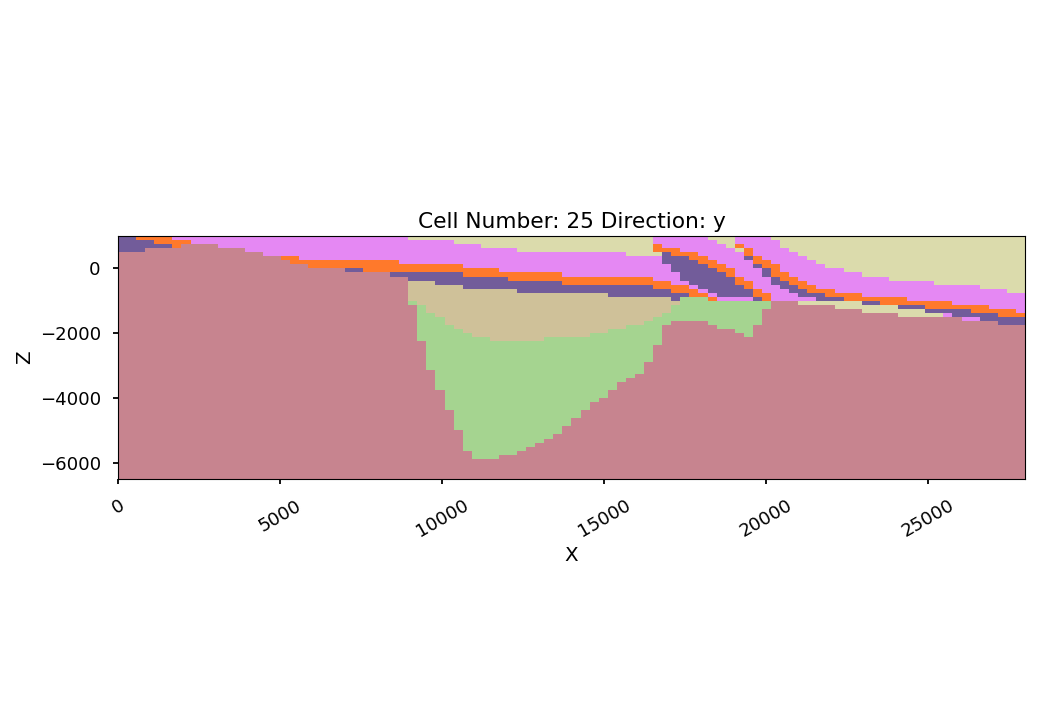
Now that the model is computed, lets have a look at a cross-section along the y-axis, so across the graben system:
gp.plot_2d(geo_model, cell_number=25, direction='y', show_data=False, show_topography=False,
          show_lith=True, show_results=True, show_boundaries=False);
Out:
<gempy.plot.visualization_2d.Plot2D object at 0x0000017585940A60>
The two distinct domains in this model are directly visible: (i) the old graben system (extensional regime), covered by the (ii) thrusted, younger units.
Add Gravity grid
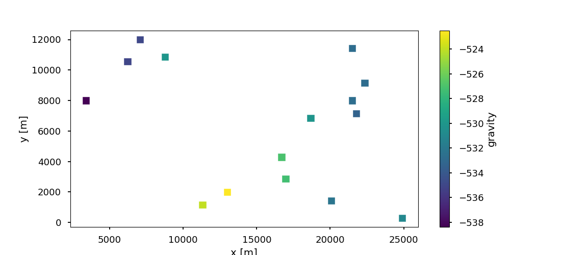
In the previous example, next to creating the model, we chose quasi-random locations for 15 gravity stations. The gravity signal of the base POC-model is simulated at these 15 stations. In the following workflows, we assume that these 15 stations were measured. So they serve as observed data for conditioning the MonteCarlo Ensemble of different geological geometries.
# In[7]:


grav_stations = pd.read_csv('../../data/Data_for_MC/20210322_forw_grav_seed58.csv')
station_coordinates = np.stack((grav_stations.X.values,
                                grav_stations.Y.values,
                                grav_stations.Z.values), axis=1)

fig = plt.figure(figsize=[11,5])
cb = plt.scatter(grav_stations['X'], grav_stations['Y'], c=grav_stations['grav'],
           marker='s', s=90, cmap='viridis')
plt.colorbar(cb, label='gravity')
plt.ylabel('y [m]')
plt.xlabel('x [m]');
Out:
Text(0.5, 13.944444444444438, 'x [m]')
These stations are used for creating a centered grid around each station. The centered grid has an extent of 10 cells in x- and y-direction, and 15 cells in the z-direction.
geo_model.set_centered_grid(station_coordinates,  resolution = [10, 10, 15], radius=6000)
g = GravityPreprocessing(geo_model.grid.centered_grid)
tz = g.set_tz_kernel()
Out:
Active grids: ['regular' 'topography' 'centered']
We see that there are three active grids. On each, the gravity signal will be calculated. Of course, we can let it be calculated on each grid, but we may not need the information on e.g. the topography grid (which would for instance yield the geological map). So we can set only the centered grid to active, which speeds up the simulation.
Note that you’ll need to model also the regular grid, if you plan to export the lith_block geological voxel model later on! As we want to also have the geometric changes in the lithological grid, we set reset=False. If we were to set it to True, only the ‘centered’ grid would be active.
geo_model.set_active_grid('centered', reset=False)
Out:
Active grids: ['regular' 'topography' 'centered']

Grid Object. Values:
array([[  140.        ,   140.        , -6437.5       ],
       [  140.        ,   140.        , -6312.5       ],
       [  140.        ,   140.        , -6187.5       ],
       ...,
       [30888.89      ,  6285.71      , -3495.98176905],
       [30888.89      ,  6285.71      , -4948.49684561],
       [30888.89      ,  6285.71      , -6966.76      ]])
The centered grid will now be the only one where the model information is stored, meaning less computational time. Let’s have a look how this comes in handy, when we start to modify the depth of units and calculate the gravity.
Before running the simulations, we need to assign densities to the rock units, otherwise it will raise an error.
MC Variation
For varying the depth of units, we extract the indices of the units whose input points we want to modify. To guarantee that we always vary the original depth in each realization (and not the depth used in the previous realization), we first generate an initial-depth array, containing the original depth information of all input points:
Z_init = geo_model.surface_points.df['Z'].copy()
Having all the undisturbed depth values, we extract all surface points belonging to the units whose inputs we want to vary:
graben_lower = geo_model.surface_points.df.query("surface=='Lower-filling'")
graben_middle = geo_model.surface_points.df.query("surface=='Upper-filling'")
unconformity = geo_model.surface_points.df.query("surface=='Unconformity'")
Before running the Monte Carlo simulations, we set up the interpolator for a “fast-run”, i.e. it optimizes runtime on cost of compilation time:
gp.set_interpolator(geo_model, output=['gravity'],
                    theano_optimizer='fast_run',
                    update_kriging=True)
Out:
Setting kriging parameters to their default values.
Compiling theano function...
Level of Optimization:  fast_run
Device:  cpu
Precision:  float64
Number of faults:  5
Compilation Done!
Kriging values:
                                          values
range                                   32190.8
$C_o$                               2.46726e+07
drift equations  [3, 3, 3, 3, 3, 3, 3, 3, 3, 3]

<gempy.core.interpolator.InterpolatorModel object at 0x0000017586B9C340>
Now we are good to go and run the Monte Carlo simulation. In the following, we fix a numpy random number seed so that this MC-simulation is reproducible Then, we create empty arrays and dictionaries for the lithologies and gravity, respectively. In a for loop, we then vary depths of interface points and compute a model.
np.random.seed(1)
# allocate array for lithology blocks
lith_blocks = np.array([])
# create a dictionary to store gravity of simulations
grav = dict()
# get indices where the variable input points are
Lgraben = list(graben_lower.index)
Ugraben = list(graben_middle.index)
Uncon = list(unconformity.index)
Cindices = Lgraben + Ugraben + Uncon

# set number of realizations
n_iterations = 10

for i in range(n_iterations):
    # vary surface points
    Z_var = np.random.normal(0, 300, size=3)
    Z_loc = np.hstack([Z_init[Lgraben] + Z_var[0],
                       Z_init[Ugraben] + Z_var[1],
                       Z_init[Uncon] + Z_var[2]])
    # apply variation to model
    geo_model.modify_surface_points(Cindices, Z=Z_loc)
    # re-compute model
    gp.compute_model(geo_model)
    # store lithologies ONLY THERE IF REGULAR GRID IS ACTIVE
    lith_blocks = np.append(lith_blocks, geo_model.solutions.lith_block)
    # store gravity
    grav[f"Real_{i}"] = geo_model.solutions.fw_gravity

lith_blocks = lith_blocks.reshape(n_iterations, -1)
Export models and gravity
For post-processing of use in different software (e.g. numerical simulators for heat- and mass-transport), knowing ways of exporting the MC-results, in this case the simulated gravity and the lithology-blocks, comes in handy. There are many different ways of saving stuff (e.g. pickle the simulation results), but here we present simple exports as .csv and .npy files.
gravdf = pd.DataFrame.from_dict(grav)

# add station coordinates to the dataframe
gravdf["X"] = station_coordinates[:,0]
gravdf["Y"] = station_coordinates[:,1]
gravdf["Z"] =station_coordinates[:,2]

gravdf.head()
This can be saved as usual with df.to_csv(‘pathname’) using Pandas. For the lithological block model, one good option is to save it as a numpy array, using numpy.save().
np.save('../../data/outputs/MCexample_10realizations.npy', lith_blocks)
Quick model analysis
Let’s have a quick first look at the resulting gravity and lithological block models. From the gravity dictionary, we can quickly generate a dataframe, convenient for further model analysis.
prob_block = gp.bayesian.fields.probability(lith_blocks)
ie_block = gp.bayesian.fields.information_entropy(prob_block)
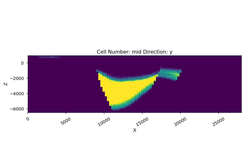
The following plot shows the probability of unit 5 in the probability block. With faults not being excluded, and counting of units starting with 0, we can see that the index 5 relates to the Lower-filling surface. The plot shows where to expect the unit. Everywhere, this unit is present throughout the simulations, the probability plot shows a bright yellow (probability = 1). Where it is always absent, we see the dark violet (probability = 0). The blueish-greenish areas are in between, meaning that in some realizations, the Lower-filling unit is present there, in other realization it is not.
layer = 5
gp.plot_2d(geo_model,
            show_lith=False, show_boundaries=False, show_data=False,
            regular_grid=prob_block[layer],
            kwargs_regular_grid={'cmap': 'viridis',
                                 'norm': None}
            );
Out:
<gempy.plot.visualization_2d.Plot2D object at 0x0000017586724700>
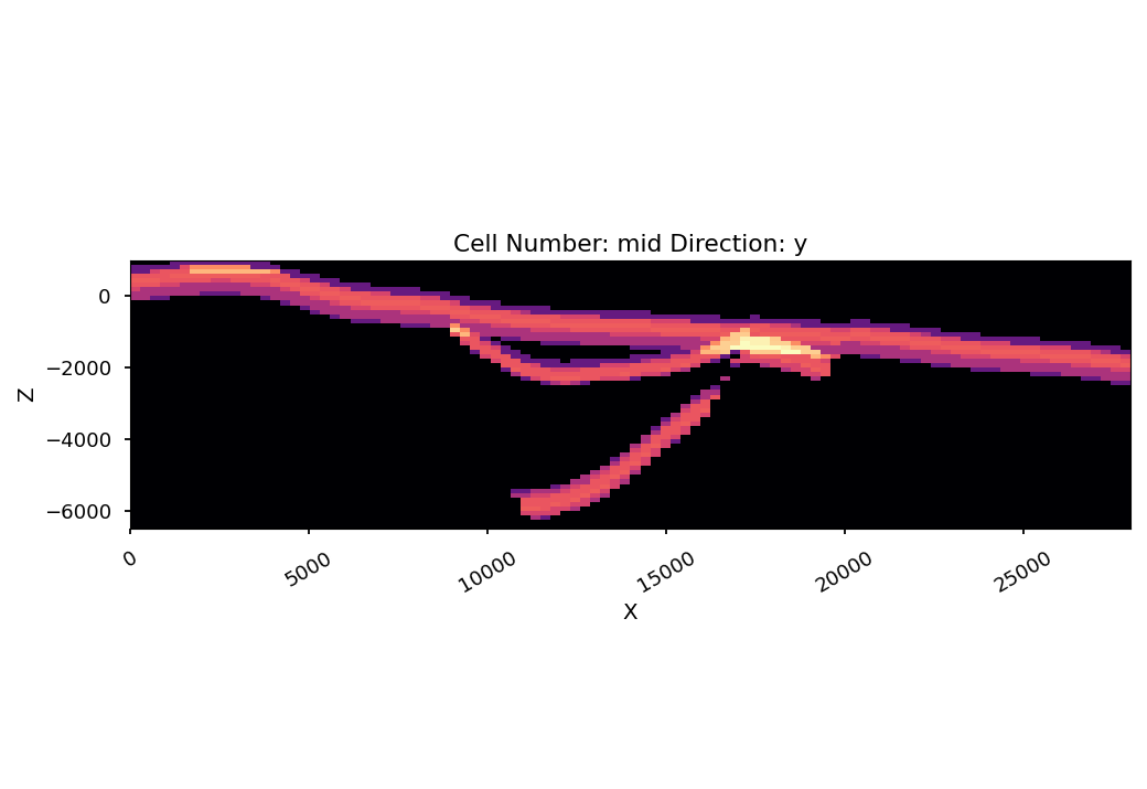
In the for-loop above, we not only varied the bottom boundary of the Lower-filling unit, but also Upper-filling and Unconformity. Using the measure of information entropy, we can visualize the parts of the model, where the most change is happening, i.e. where entropy is largest. Black areas in the following plot have zero information entropy, as there is only one “microstate” for the system, i.e. the model ensemble.
This means, we’d always encounter the same unit at the same place in every ensemble member. The colored areas, however, are areas where we’d encounter different geological units between ensemble members.
gp.plot_2d(geo_model,
            show_lith=False, show_boundaries=False, show_data=False,
            regular_grid=ie_block,
            kwargs_regular_grid={'cmap': 'magma',
                                 'norm': None}
            );
Out:
<gempy.plot.visualization_2d.Plot2D object at 0x0000017581AF3F10>
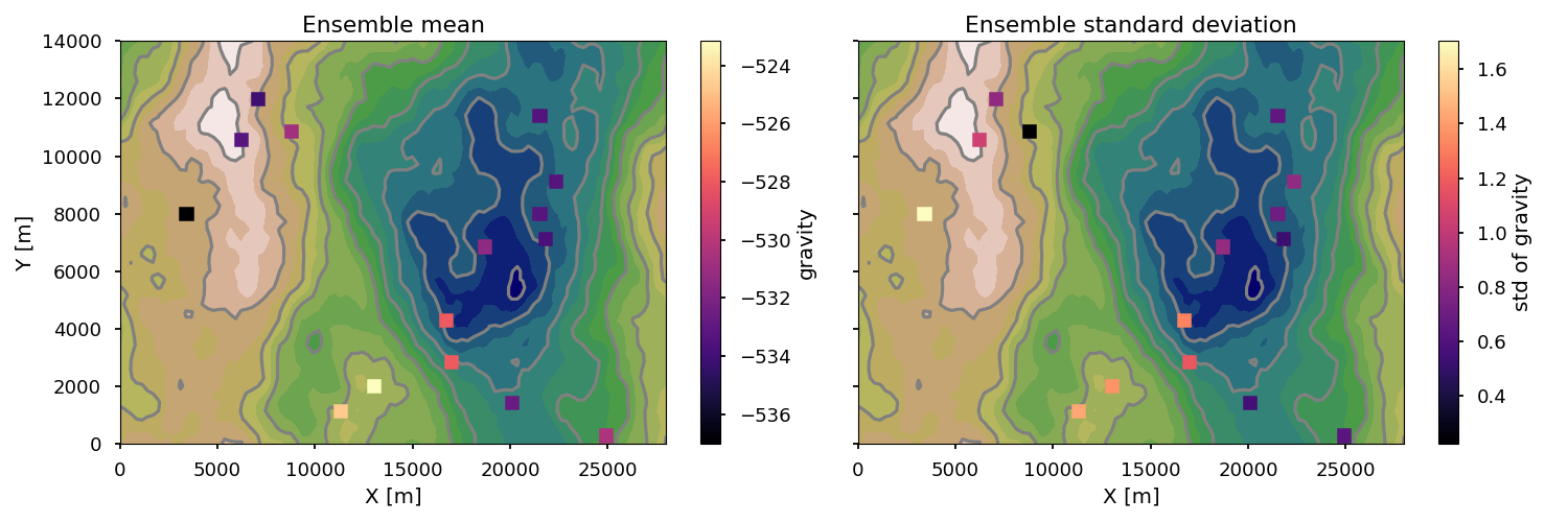
Finally, let’s have a look at the gravity. We’ll simply have a look at mean and standard deviation of the simulated gravity of the ensemble:
# make subplots with mean and std
gravdf_plt = pd.DataFrame.from_dict(grav)
gravdf_plt.to_csv('../../data/outputs/MCexample_10grav.csv', index=False)

fig, axs = plt.subplots(1,2, figsize=[15,5], sharey=True)
m_grav = np.mean(gravdf_plt, axis=1)
st_grav = np.std(gravdf_plt, axis=1)

m = axs[0].scatter(grav_stations['X'], grav_stations['Y'], c=m_grav,
           marker='s', s=90, cmap='magma', zorder=2)
axs[0].contourf(dtm[:,:,0], dtm[:,:,1], dtm[:,:,2],20, cmap='gist_earth', zorder=0)
axs[0].contour(dtm[:,:,0], dtm[:,:,1], dtm[:,:,2],10, colors='gray', zorder=1)
s = axs[1].scatter(grav_stations['X'], grav_stations['Y'], c=st_grav,
              marker='s', s=90, cmap='magma', zorder=2)
axs[1].contourf(dtm[:,:,0], dtm[:,:,1], dtm[:,:,2],20, cmap='gist_earth', zorder=0)
axs[1].contour(dtm[:,:,0], dtm[:,:,1], dtm[:,:,2],10, colors='gray', zorder=1)
fig.colorbar(m, ax=axs[0], label='gravity')
fig.colorbar(s, ax=axs[1], label='std of gravity')
axs[0].set_title('Ensemble mean')
axs[1].set_title('Ensemble standard deviation')
axs[0].set_ylabel('Y [m]')
axs[0].set_xlabel('X [m]')
axs[1].set_xlabel('X [m]')

fig.tight_layout()
Total running time of the script: ( 4 minutes 54.026 seconds)
