Note
Click here to download the full example code
01 - Geological model creation and gravity simulation
The following tutorial will step-by-step lead you through an example workflow on creating a GemPy model from interface and orientation data, assigning densities to geological units, and model their gravity response.
Create the base Proof-of-Concept Model
Based on a seismic section from the NAGRA report NAGRA NAB 14-17 [1], we extracted interface and orientation points for lithological units and faults.
The lithological units comprise the permo-carboniferous filling (divided in three stages based on the report results), Mesozoic, Tertiary, and Quaternary strata, as well as the Palaeozoic crystalline basement rocks.
import warnings
warnings.filterwarnings("ignore")

# Importing GemPy
import gempy as gp
from gempy.plot import visualization_2d as vv

# Importing auxilary libraries
import numpy as np
import pandas as pd
import matplotlib.pyplot as plt
plt.style.use('seaborn-talk')

# What GemPy version was used
print(f"Code run with GemPy version: {gp.__version__}")
Out:
Code run with GemPy version: 2.2.9
Initialize the model
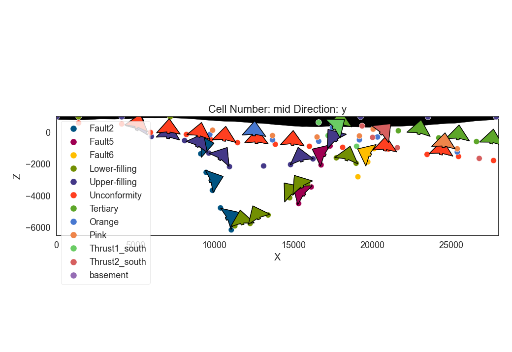
We start with modelling the trough by generating a gempy model object. This will use interface points and orientations, which we previously stored in a .csv file.
# Fix random number seed to get the same topography
np.random.seed(333)
# Import data
# Create a model instance
geo_model = gp.create_model('POC_model')

# Initialize the model, set dimension and load interface and orientation data
gp.init_data(geo_model, [0, 28000., 0, 14000., -6500, 1000.], [100, 50, 60],
            path_i = '../../data/GemPy/line82_interfaces_wo_middle_MC.csv',
            path_o = '../../data/GemPy/line82_foliations_wo_middle_MC.csv')
geo_model.set_topography(source='random', d_z=np.array([300,1000]))

gp.plot_2d(geo_model, show_data=True, show_topography=True)

Out:
Active grids: ['regular']
Active grids: ['regular' 'topography']

<gempy.plot.visualization_2d.Plot2D object at 0x00000175FAE709A0>
Adding information to the model
Only loading interface and orientation points is not enough. First, let’s assign colors to the different model units, e.g. for coloring faults similarly.
col_dict = {'basement': '#c7848f',
           'Lower-filling': '#a5d490',
           'Upper-filling': '#cfc199',
           'Unconformity': '#725c9a',
           'Orange': '#ff792b',
           'Pink': '#e588f3',
           'Tertiary': '#dbdbac',
           'Fault2': '#015482',
           'Fault5': '#015482',
           'Fault6': '#015482',
           'Thrust1_south': '#5DA629',
           'Thrust2_south': '#5DA629'}
geo_model.surfaces.colors.change_colors(col_dict)
geo_model.surfaces
Model Characteristics
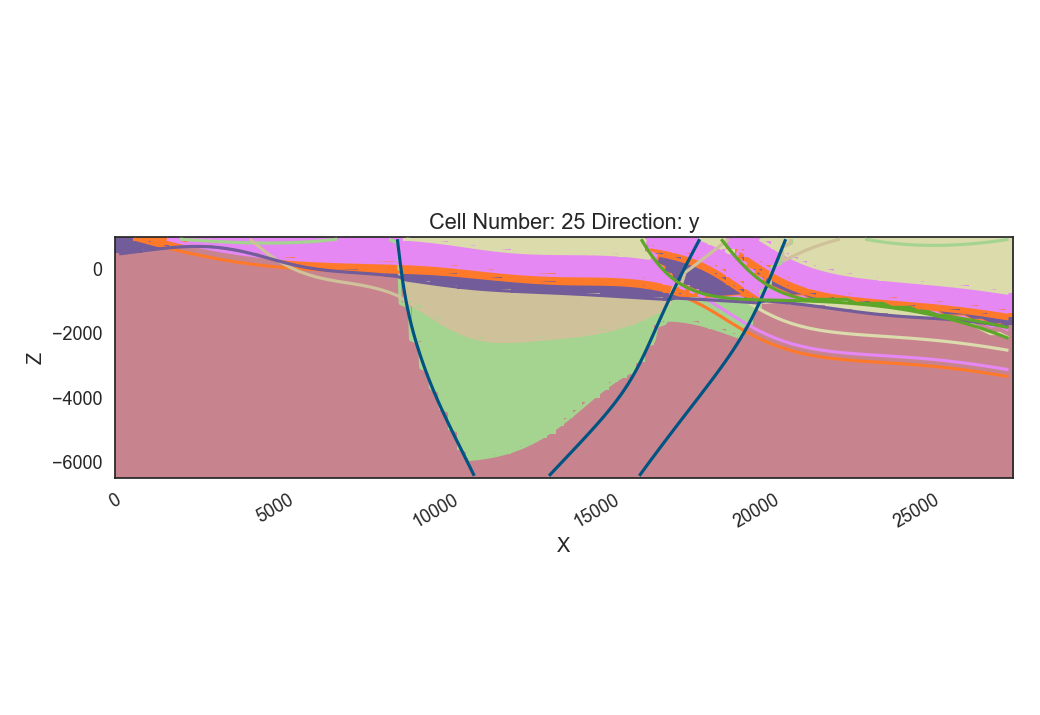
Main features of the model is the asymetric graben system, with the major fault (denoted with A), and the graben fill, which is not present beyond the graben shoulders. This, as well as the stop of major faults beneath the mesozoic units (blue units) are important considerations for the modelling process. These could be caught, for instance, in likelihood functions if we model the PCT as a Bayesian inference problem.
# Assign formations to series
gp.map_series_to_surfaces(geo_model,
                         {"Thrust1_series": 'Thrust1_south',
                          "Thrust2_series": 'Thrust2_south',
                          "Fault2_series": 'Fault2',
                          "Fault5_series": 'Fault5',
                          "Fault6_series": 'Fault6',
                         "Post_tectonic_series": ('Tertiary', 'Pink', 'Orange'),
                          "Detachement": 'Unconformity',
                         "Syn_tectonic_series2": 'Upper-filling',
                         #"Syn_tectonic_series1": 'Middle-filling',
                         "Pre_tectonic_series": 'Lower-filling'},
                         remove_unused_series=True)
geo_model.surfaces
After assigning units to stacks or series, we have so define which of those series is a fault. Here, we see that it is usually important to assign each fault its own series, as faults may have very different scalar fields (in which the fault surfaces are interpolated).
geo_model.set_is_fault(['Thrust1_series', 'Thrust2_series',
                        'Fault2_series', 'Fault5_series', 'Fault6_series'],
                      change_color=False)
Further we have to set bottom relations, if a series is not erosive. For instance, the Units in the Graben are most likely onlapping units.
geo_model.set_bottom_relation(series=['Post_tectonic_series',
                                      'Pre_tectonic_series',
                                      'Syn_tectonic_series2'], bottom_relation='Onlap') #,
The following table shows the fault relations, i.e. which unit (or fault) is affected by a fault. If the respective entry in the table is set to True, the fault on the left displaces the unit (or fault) in a respective column.
geo_model.faults.faults_relations_df
Per default, faults displace all lithological units. However, the normal faults of the graben do not affect the younger units, so we define a boolean matrix, which sets the fault relations correctly.
fr = np.array([[False, True, False, False, False, True, False, False,   False, False],
               [False, False, False, False, False, True, False, False,  False, False],
               [False, False, False, False, False, False, True, True,  True, True],
               [False, False, False, False, False, False, True, True,  True, True],
               [False, False, False, False, False, False, True, True,  True, True],
               [False, False, False, False, False, False, False, False, False, False],
               [False, False, False, False, False, False, False, False, False, False],
               [False, False, False, False, False, False, False, False, False, False],
               [False, False, False, False, False, False, False, False, False, False],
               [False, False, False, False, False, False, False, False, False, False]])
geo_model.set_fault_relation(fr)
Creating the model
Now that we set the parameters and fault relations, it is time to start the modeling process:
# decrease the kriging range
geo_model.modify_kriging_parameters('range', 20000.)
geo_model.modify_kriging_parameters('$C_o$', 2e5)

# Set the interpolator function
gp.set_interpolator(geo_model,
                         compile_theano=True,
                         theano_optimizer='fast_compile',
                         verbose=[],
                         update_kriging=False)

# Compute the model
sol = gp.compute_model(geo_model)
Out:
Compiling theano function...
Level of Optimization:  fast_compile
Device:  cpu
Precision:  float64
Number of faults:  5
Compilation Done!
Kriging values:
                                          values
range                                     20000
$C_o$                                    200000
drift equations  [3, 3, 3, 3, 3, 3, 3, 3, 3, 3]
Saving the model is straight forward. It can optionally also be compressed in a zip archive, or be _pickled_. An example on how to save a model is shown next. There, we give the saving path and the model name.
geo_model.save_model(name='POC_PCT_model',
                     path='../../models/2021-06-04_POC_base_model')
Out:
True
Let’s have a look how the created model looks like:
gp.plot_2d(geo_model, cell_number=25, direction='y', show_data=False, show_topography=False,
          show_lith=True, show_results=True, show_boundaries=True)

Out:
<gempy.plot.visualization_2d.Plot2D object at 0x00000175860F79D0>
The displayed lithologies are stored in a regular grid, which we defined at the beginning. We can store this grid, containing the lithology IDs in space for further postprocessing
np.save('../../models/POC_base_model_lith_blocks.npy', np.round(geo_model.solutions.lith_block,0).astype('int'))
Simulate Gravity
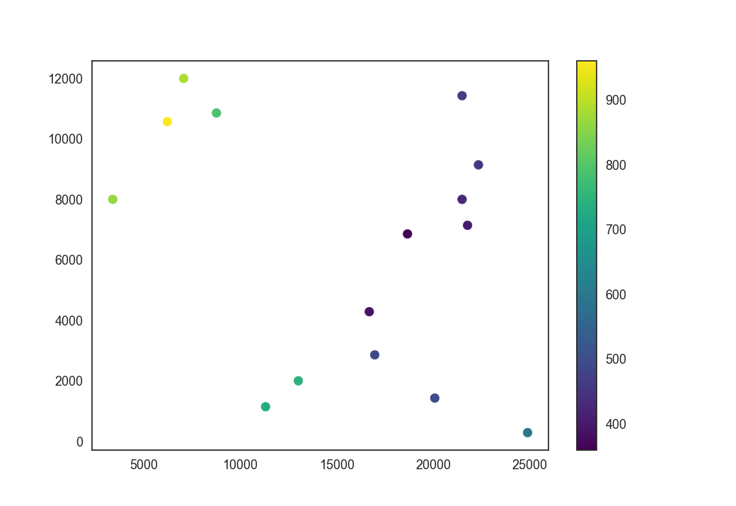
Using the now generated POC-model, we simulate its gravity at different locations. These locations will be treated as observations later on in the workflow. In a first step, we distribute 15 points randomly across the topography of our model. Those will be the station locations, where we pick up the gravity signal of the POC-model.
# distribute stations
import random
np.random.seed(58)
station_indices = np.random.randint(0, high=4999, size=15)
station_coordinates = geo_model._grid.topography.values[station_indices, :]

cs = plt.scatter(station_coordinates[:,0], station_coordinates[:,1], c=station_coordinates[:,2], cmap='viridis')
plt.colorbar(cs)

Out:
<matplotlib.colorbar.Colorbar object at 0x0000017586E85F40>
Next, we create centered grids around each station. The centered grid here has 10 cells in x- and y-direction, and extends 15 cells down in the z-direction.
from gempy.assets.geophysics import GravityPreprocessing
geo_model.set_centered_grid(station_coordinates,  resolution = [10, 10, 15], radius=6000)
g = GravityPreprocessing(geo_model.grid.centered_grid)
tz = g.set_tz_kernel()
Out:
Active grids: ['regular' 'topography' 'centered']
The gravity response cannot be modeled without assigning a density to the model units. Theoretically, one could also assign different petrophyiscal properties here. They will be added as separate columns to the surfaces dataframe.
Modeling the lithology on all grids (regular, topography, centered) can get time consuming. So here, we only activate the centered grid to catch the gravity response.
geo_model.set_active_grid('centered', reset=True)

gp.set_interpolator(geo_model, output=['gravity'], theano_optimizer='fast_run', update_kriging=False)
sol = gp.compute_model(geo_model)
# reshape solved gravity and add coordinates
grav = sol.fw_gravity
grav1 = grav.reshape(len(grav),1)
station_forw_grav = np.round(np.append(station_coordinates, grav1, axis=1),4)
# make everything into a dataframe
df_stations = pd.DataFrame(station_forw_grav, columns=["X", "Y", "Z", "grav"])
# round X Y and Z to 2 decimals
df_stations[['X','Y','Z']] = np.around(df_stations[['X','Y','Z']], 2)
Out:
Active grids: ['centered']
Compiling theano function...
Level of Optimization:  fast_run
Device:  cpu
Precision:  float64
Number of faults:  5
Compilation Done!
Kriging values:
                                          values
range                                     20000
$C_o$                                    200000
drift equations  [3, 3, 3, 3, 3, 3, 3, 3, 3, 3]
and finally, we save the modeled gravity to be used as observations later on:
df_stations.to_csv('../../data/Data_for_MC/20210322_forw_grav_seed58.csv', index=False)
References
[1] Naef, H., & Madritsch, H. (2014). Tektonische Karte des Nordschweizer Permokarbontrogs: Aktualisierung basierend auf 2D-Seismik und Schweredaten. Nagra Arbeitsbericht (NAB 14-17). Wettingen: Nagra.
Total running time of the script: ( 0 minutes 59.426 seconds)
