Usage

Prerequisites

Before running, ensure that you have completed a reservoir simulation and that the output includes all necessary data for flow diagnostics. This should include pore volume, fluxes, cell connections, and well information, stored in the binary output files.

• For SLB simulators (or OPM): ensure that you generate .INIT and .EGRID files. Additionally, specify FLORES under RPTPST keyword to output fluxes in reservoir conditions. Alternatively, the tool also works if both fluxes in surface conditions and formation volume factors are available.

• For CMG simulators: Use FLUXCON along with OUTSRF keyword to output fluxes in reservoir condition.

Running the tool

Via the command line:

pyflowdiagnostics -f <PATH_TO_DATA/AFI_FILE> -t <LIST_OF_TSTEPS_OF_INTEREST>

Arguments:

• -f <PATH_TO_SIMULATOR_PRIMARY_INPUT_FILE>: Path to the reservoir simulation primary input file (.DATA, .AFI, or .DAT).

• -t <LIST_OF_TSTEPS_OF_INTEREST>: List of reservoir simulation output (grid dynamic simulation results) time step indices to run the diagnostics on.

• -d: An optional argument to enable debug mode.

Example

Using command line interface (CLI):

pyflowdiagnostics -f /path/to/simulation.DATA -t 1 5 10

Or, in your Python script:

import pyflowdiagnostics as pfd

tsteps = [1, 5, 10]

fd = pfd.FlowDiagnostics("/path/to/simulation.DATA")
for tstep in tsteps:
    fd.execute(tstep)

The code will identify the simulator type based on the file path (extension) and then use appropriate binary reader.

Output

The script generates a folder named CASENAME.fdout in the same directory as the provided DATA/AFI/DAT file. This folder contains:

• Grid flow diagnostics results (time-of-flight, flow partitioning, well pair IDs) in Petrel readable (.GRDECL) format.

• If applicable:

  • Allocation factors.

  • Lorentz curve data.

  • Sweep efficiencies.

Sample results:

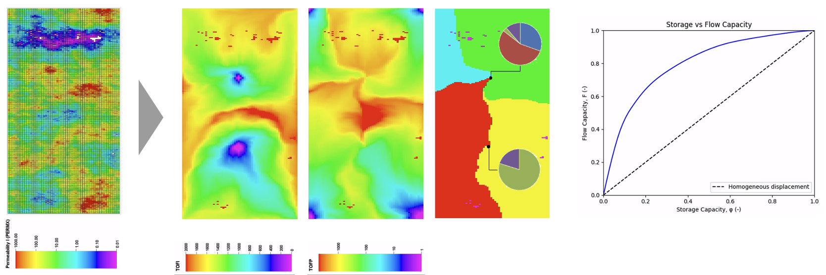
SPE10 top layer: TOF, flow partition, allocation factors, Lorentz curve.

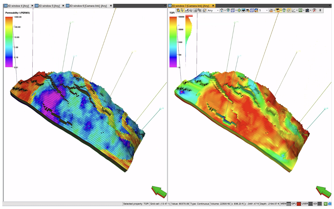
SAIGUP: permeability and TOF.